NOMAD Observation and Measurement Types

NOMAD can make a wide variety of observations, for example occultation, dayside nadir, limb, etc; and for each observation it can measure in one of many different measurement types. This page aims to:

Explain how each observation/measurement type is made
Give a list of possible advantages/disadvantages and limitations of each type
Explain how the data pipeline processes the data
Describe how the data is stored within the hdf5 files made available to the science team

Observation Types

Observation Types	Description
Ingress solar occultation	Normal solar occultation starting when the line of sight is above the atmosphere and ending when sun is blocked by the surface
Egress solar occultation	Normal solar occultation starting when the line of sight to the sun is blocked by the surface and ending when it is above the atmosphere
Merged solar occultation	Double solar occultation, consisting of an ingress, starting above atmosphere, and an egress, ending above atmosphere. These occur when there is insufficient time between the ingress and egress to cool down the infrared detector for the second measurement
Grazing solar occultation	Solar occultation where, due to orbital geometry, the sun is never blocked by the surface. Starting above the atmosphere, the line of sight passes through the atmosphere to a minimum altitude, then increases to end above the atmosphere
Dayside Nadir	Nadir measurement on the illuminated side of the planet. Observations can be of variable length, beginning and ending near the nightside terminator to cover the whole dayside, or shorter and centred on the subsolar latitude. Can also be split into 3 separate measurements
Nightside Nadir	Nadir measurement on the nightside of the planet
Limb	Measurement of the illuminated limb of the planet
Calibration	Many types e.g. sun pointing, solar line scan, etc.

Measurement Types

Measurement Types - SO/LNO Channels	Description
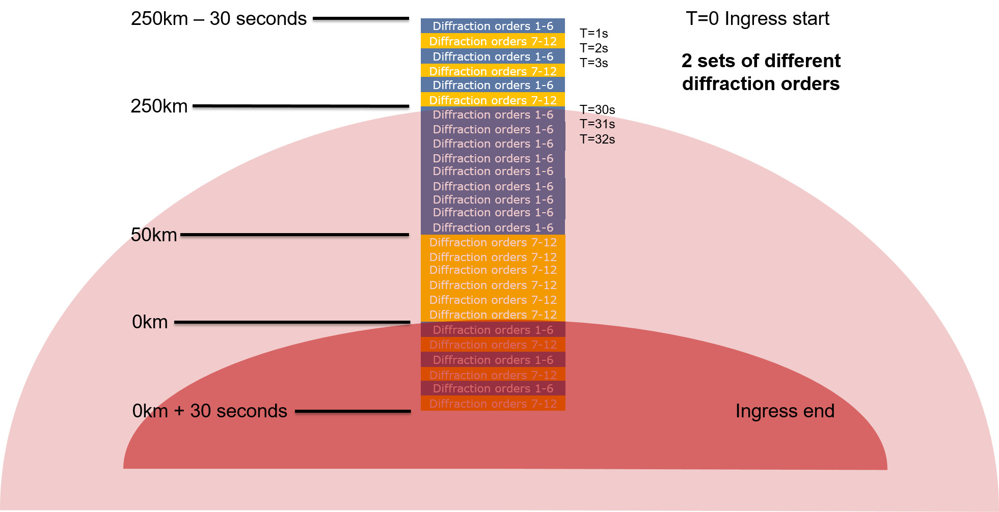
Solar occultation (50km switch)	5 diffraction orders + 1 dark per second. When the line of sight reaches 50km , the combination of diffraction orders being measured is changed. No onboard background subtraction
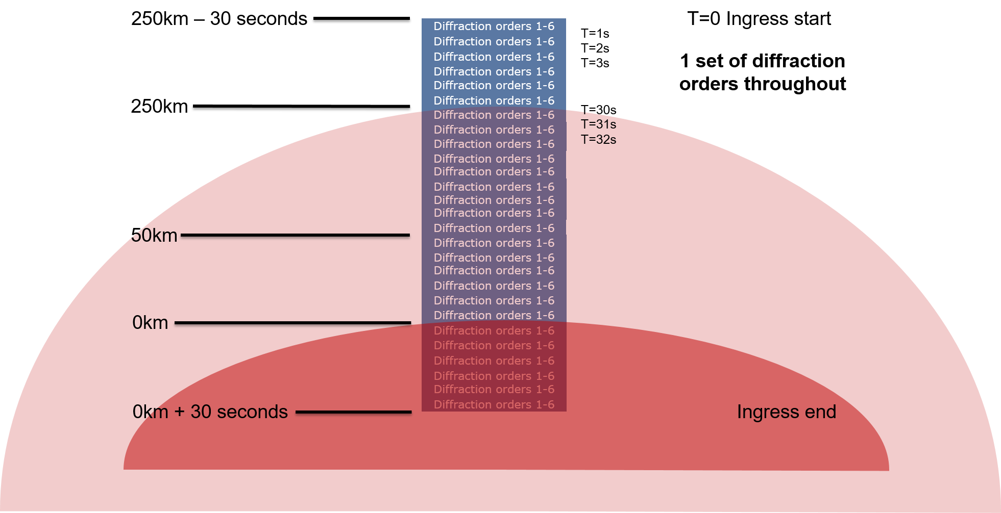
Solar occultation (0-250km)	5 diffraction orders + 1 dark per second, same order selection throughout. No onboard background subtraction
Solar occultation (50km switch, dark subtraction)	6 diffraction orders per second, diffraction order selection changed at 50km. Dark frames subtracted onboard
Solar occultation (0-250km, dark subtraction)	6 diffraction orders per second, same order selection throughout. Dark frames subtracted onboard
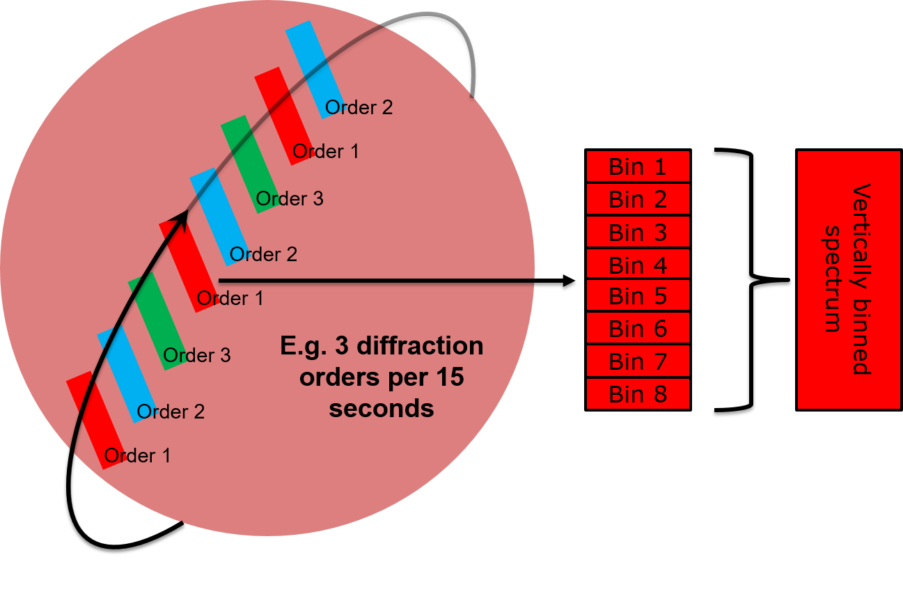
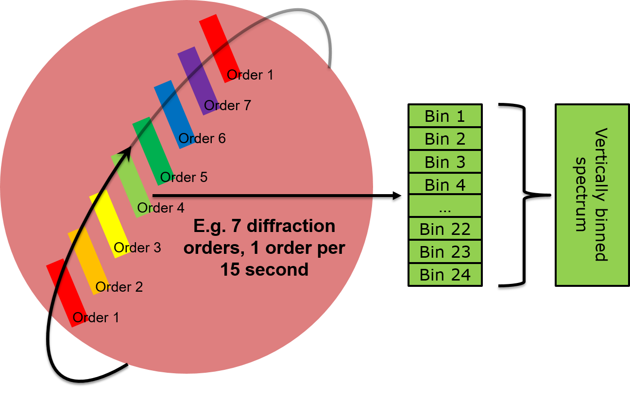
Nadir	Nadir measurement of 2 to 6 diffraction orders per 15 seconds, dark subtracted onboard
Limb	Limb measurement of 2 diffraction orders per 15 seconds, dark subtracted onboard
ACS Boresight Limb	Special limb measurement of 2+ diffraction orders, measured during an ACS/MIR or ACS/TIRVIM solar occultation where line of sight is pointed close to the sun but not directly at the solar disk. Onboard dark subtraction
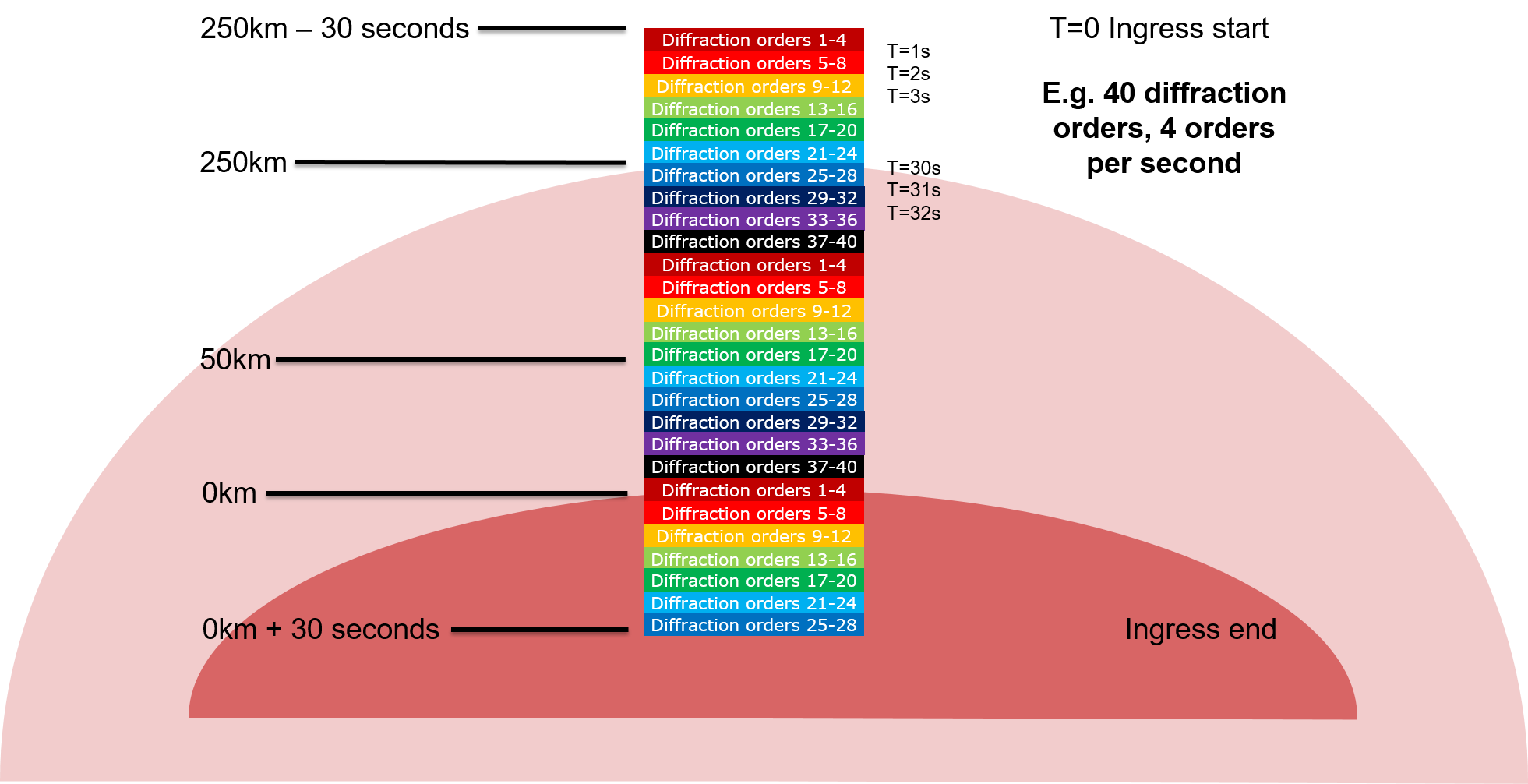
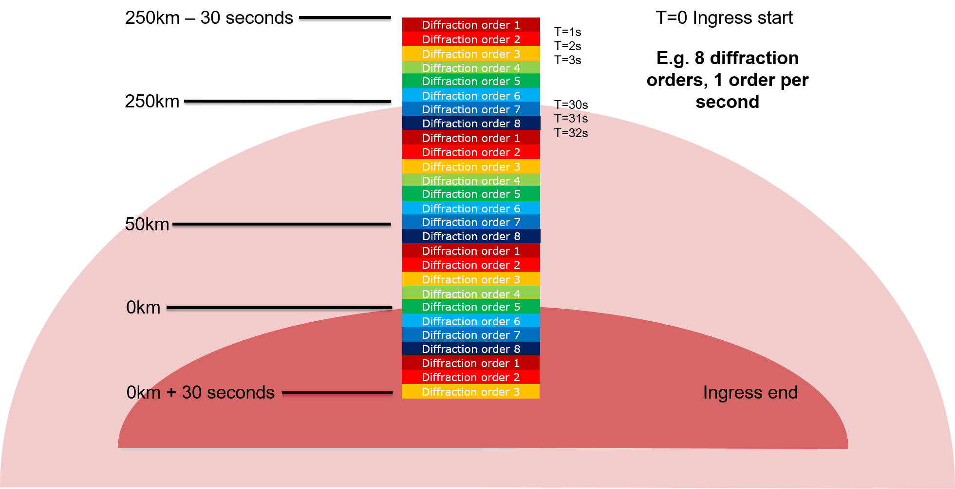
Fullscan (slow)	Nadir, limb or occultation diffraction order stepping over any range/number of orders, dark subtracted onboard
Fullscan (fast)	Solar occultation order stepping over any range/number of orders at a high cadence rate, dark subtracted onboard
Calibration	Many types e.g. line of sight, solar fullscan, solar miniscan, integration time stepping, etc.
Measurement Types - UVIS Channel	Description
Solar occultation (binned)	Detector pixel values are vertically binned onboard. 3 full or partial spectra are recorded per second. No dark subtraction is made onboard
Solar occultation (unbinned)	Each pixel value is stored individually. Full or partial spectra can be transmitted to Earth at a variety of cadence rates. No dark subtraction is made onboard
Nadir (binned)	Detector pixel values are vertically binned onboard. Full or partial spectra can be transmitted to Earth at a variety of cadence rates. Occasional dark frames are taken and transmitted to Earth
Nadir (unbinned)	Each pixel value is stored individually. Full or partial spectra can be transmitted to Earth at a variety of cadence rates. Occasional dark frames are taken and transmitted to Earth
Calibration	Many types e.g. line of sight, integration time tests, etc.

Data Pipeline Processing of Observations

Every HDF5 file has an observation type letter in its name. As can be seen above, there are many many possible combinations of observation and measurement types; far too many to assign a letter to each. The observation type letter can be used to find certain observation types, but the primary use is to direct the file through the correct branch of the data processing pipeline.

Below is a description of each type of observation/measurement type and what steps are taken to convert the raw telemetry into a calibrated HDF5 file.

Observation Type(s)	Ingress Solar Occultation	Egress Solar Occultation
Measurement Type(s)	SO Solar Occultation (50km switch)	SO Solar Occultation (0-250km)
Processing Step(s)	Level 0.1A Housekeeping calibration Level 0.1D Split by diffraction order Expand filenames Level 0.1E Non-linearity Bad pixel Level 0.2A Solar occultation geometry Level 0.3A Infrared spectral calibration Level 1.0A Transmittance calibration

Observation Type(s)

Ingress Solar Occultation

Egress Solar Occultation

Measurement Type(s)

SO Solar Occultation (50km switch)

SO Solar Occultation (0-250km)

Processing Step(s)

Observation Type(s)	Dayside Nadir	Nightside Nadir
Measurement Type(s)	UVIS nadir (unbinned)	UVIS nadir (binned)
Processing Step(s)	Level 0.1A Housekeeping calibration Level 0.2A Nadir geometry Level 0.3B UVIS reshape dataset UVIS dynamic range correction UVIS detector saturation detection Level 0.3C UVIS dark current removal UVIS anomaly detection Level 0.3D UVIS spectral calibration Level 0.3E UVIS straylight removal

Observation Type(s)

Dayside Nadir

Nightside Nadir

Measurement Type(s)

UVIS nadir (unbinned)

UVIS nadir (binned)

Processing Step(s)

Level 0.1A

Housekeeping calibration

Level 0.2A

Nadir geometry

Level 0.3B

UVIS reshape dataset
UVIS dynamic range correction
UVIS detector saturation detection

Level 0.3C

UVIS dark current removal
UVIS anomaly detection

Level 0.3D

UVIS spectral calibration

Level 0.3E

UVIS straylight removal

Level 0.1A

Housekeeping calibration

Conversion of housekeeping to physical units

Level 0.1D

Split by diffraction order

All SO/LNO files, except fullscans, are split into one file per diffraction order. If the diffraction orders are switched at 50km, then two sets of files are created, appended by the OrderSet (_1 or _2, where 1 is chronologically first).

Expand filenames

Observation type letter and diffraction order added to filename. Naming now follows the following convention:

YYYYMMDD_hhmmss_Level_Channel_OrderSet_ObservationTypeLetter_DiffractionOrder.h5

YYYY is the observation start year
MM is the observation start month
DD is the observation start date
hh is the observation start time hour
mm is the observation start time minute
ss is the observation start time second
Level is the data level with a letter p to replace the point, e.g. 0p1a, 0p3a, 1p0a, etc.
Channel is either SO, LNO or UVIS
(SO/LNO only) OrderSet is either 1 or 2 indicating the set of diffraction orders used. The orders can change during an occultation, therefore the first set is 1 and the second set is 2. If the same order combination is used throughout, this is always 1.
ObservationTypeLetter is defined here
(SO/LNO only and not for fullscans) DiffractionOrder is the diffraction order

Level 0.1E

LNO straylight

Straylight can be observed in the data when the LNO channel is observing in nadir and the spacecraft is in a particular geometry which only occurs when slewing to an ACS solar occultation. This happens only on the nightside of the planet and so no science is lost. However, a signal is observed in the data, and so the affected frames are removed to avoid misinterpretation of the spectra.

Frames containing this straylight are removed automatically, based on a set of detection criteria - i.e. spacecraft orientation with respect to the Sun, and anomalous detector values. The frames directly before and after are also removed, to ensure that all incorrect data is removed.
The data is not recoverable when straylight is present, and so all data in the affected frames in Science/Y are set to NaN. The filed Science/YValidFlag is used to indicate which spectra are valid, where:

1 = spectrum is valid
0 = spectrum is invalid

The data therefore is in the following format, assuming straylight has been detected in measurement frame 4:

Science/Y
Measurement 1, Pixel 1 Value	Pixel 2 Value	...	Pixel 320 Value
Measurement 2, Pixel 1 Value	Pixel 2 Value	...	Pixel 320 Value
NaN	NaN	...	NaN
NaN	NaN	...	NaN
NaN	NaN	...	NaN
Measurement 6, Pixel 1 Value	Pixel 2 Value	...	Pixel 320 Value

Science/YValidFlag
1
1
0
0
0
1

SO non-linearity

The SO and LNO detectors and readout electronics have a slightly non-linear response the radiance when the incident radiance is very small. The SO channel observes the sun during a solar occultation, and so low integration times (~4ms) are used to avoid saturation. This means that when the input radiance is low (e.g. when viewing the lower atmosphere, or planet, or when taking a dark frame) then the signal could be within the non-linear region. This never applies to nadir or limb data, as the lower signal means that the long integration times (~200ms) are required.

The correction is derived from integration time stepping measurements viewing dark space.

The integration time is stepped from 0 to 1400ms, and a linear fit is made to the data from 200-1400ms to calculate the difference between expected and measured counts in the non-linear region. This is done for every pixel individually, though the variation between pixels is very small. The figure above shows the deviation from non-linearity for a single pixel - the region is compared to the entire detector region (a pixel saturates around 12000 counts), and when zoomed in the deviation from the linear fit remains small.

Every detector count is checked to see if the value is within the non-linear region. If so, that value is replaced by the linear-equivalent value from the line of best fit.

SO/LNO bad pixel

Two methods were attempted to remove the bad pixels. The first used a bad pixel map, as above, derived from integration time stepping measurements for every pixel. Bad pixels are easily identifiable from the slope of the linearity curves and deviation from a linear fit. Pixels in white show the greatest deviation, whilst the manufacturing pattern can be seen on the remainder of the pixel. The bad pixel map defines all pixels as either bad or good, and so care must be taken to tune the cut-off value correctly to avoid missing bad pixels or adding good pixels to the bad pixel map. Three bad pixel maps were made - normal, sensitive, and very sensitive - to test the best cut-off value (where very sensitive means that pixels with even a small deviation are designated as bad pixels).

Another method is to analyse all spectra and determine the pixels that behave anomalously compared to adjacent pixels throughout a measurement. This method works even for the narrowest absorption lines, as there is always a spectral overlap between consecutive pixels, and so an anomalous value in one pixel only can only be due to the pixel, not the atmosphere or surface of Mars. As above, the detection is sensitive to the cut-off value used to define whether the behaviour of a given pixel is "good" or "bad".

Both methods described above had problems, either with bad pixels remaining in the data or good pixels being corrected. In particular, some bad pixels occur intermittently and so are missed from the first method and not picked up by the second. Instead, a hybrid approach is now used, combining the sensitive bad pixel map with a check of all spectra. If a pixel behaves anomalously and is on the list of bad pixels, then the pixel is corrected by linearly interpolating from adjacent pixels. Pixels at the edge of the detector, where the signal is already very small, are not corrected.

LNO detector offsets

The zero offset level can shift up and down due to the detector grounding and the very small values generated by a nadir measurement. To correct this, an offset correction is calculated from the mean of the first 50 pixels. The offsets are subtracted from each spectrum to remove the anomalous offset. The subtracted offset values (one per spectrum) are stored in the attribute DetectorOffsetsSubtracted.

Removing the offset means that the first pixels can be less than zero, therefore a second offset is subsequently added to the data. This offset is derived from solar calibration measurements of the same diffraction order, where a ratio is calculated between the mean of the centre pixels [160-240] and the mean of the first 50 pixels when pointing at the sun.

An offset is then added to each nadir spectrum so that the same ratio is present in the data. The added offset values (one per spectrum) are stored in the attribute DetectorOffsetsAdded.

LNO nadir data vertically binned

The applies only to LNO nadir data. The SNR of the LNO channel is low, and so the spectra measured for each detector bin (of the same measurement) and summed together to give one spectrum. All detector rows for each diffraction order are vertically binned, to give a single spectrum per measurement. The detector bins observe different locations on the planet, but this spatial information is lost when the data is binned - though individual bins do not have sufficient signal to be scientifically useful.

The SO and LNO channel always return 24 lines per measurement period (where the period is 1 second for occultation or 15 seconds for nadir observations). Therefore here, 3 orders are measured per period and so 8 spectra are returned per order. If 4 orders were measured, 6 spectra would be returned; if 2 orders then 12 spectra would be returned, etc. LNO nadir data is then orders

SO/LNO detector bins flattened

SO and LNO Science/Y datasets (except LNO nadir) are converted from a 3D array (size = number of observations x number of bins x 320 pixels) to a 2D array (size = [number of observations x number of bins] x 320 pixels). Science/Bins contains the start and bin detector row for each bin.
LNO nadir observations have already been vertically binned into a 2D array.

Level 0.2A

There are three types of shape models used to calculate geometric parameters:

Ellipsoid - this is the most basic shape model, where Mars is modelled as a tri-axial ellipsoid of radii 3396.19km x 3396.19km x 3376.2km
Areoid - this is the equivalent to a "sea level" for Mars, where the gravitational and rotational potential is constant across the entire surface. The zero level is defined by MGS/MOLA using a 4 pixels per degree model
Surface - this is the real surface elevation, calculated from a digital shape kernel (DSK) by MGS/MOLA at a resolution of 4 pixels per degree using the MGM1025 model (Lemoine et al., 2001)

Solar occultation geometry

Description

Geometry is stored for each point. There are 5 points for SO/LNO solar occultations:

Geometry/Point0 is the centre of the field of view
Geometry/Point1 to Geometry/Point4 define the corners

UVIS has a circular aperture, defined by 9 points:

Geometry/Point0 is the centre of the field of view
Geometry/Point1 to Geometry/Point8 form an octagon around the edge

Within each point are the geometry datasets. There is one row per spectrum acquired, and two columns for the start and end geometry of that acquisition:

Dataset Name	Description
Geometry/PointN/Lat
Geometry/PointN/Lon
Geometry/PointN/LOSAngle
Geometry/PointN/LST
Geometry/PointN/PointXY
Geometry/PointN/SurfaceAltAreoid
Geometry/PointN/SurfaceRadius
Geometry/PointN/TangentAlt
Geometry/PointN/TangentAltAreoid
Geometry/PointN/TangentAltSurface

Geometric parameters that do not depend on pointing direction are stored in the Geometry group. These are:

Dataset Name	Description
Geometry/DistToSun
Geometry/LSubS
Geometry/ObsAlt
Geometry/ObservationDateTime
Geometry/ObservationEphemerisTime
Geometry/SpdObsSun
Geometry/SpdTargetSun
Geometry/SubObsLat
Geometry/SubObsLon
Geometry/SubSolLat
Geometry/SubSolLon
Geometry/TiltAngle

SO/LNO Occultation (50km switch)

SO/LNO/UVIS Occultation (0-250km)

Data Format - one row per spectrum acquired

Science/Y
Measurement 1, Bin 1, Pixel 1	Pixel 2	...	Pixel 320
Measurement 1, Bin 2, Pixel 1	Pixel 2	...	Pixel 320
Measurement 1, Bin 3, Pixel 1	Pixel 2	...	Pixel 320
Measurement 1, Bin 4, Pixel 1	Pixel 2	...	Pixel 320
Measurement 2, Bin 1, Pixel 1	Pixel 2	...	Pixel 320
Measurement 2, Bin 2, Pixel 1	Pixel 2	...	Pixel 320

Science/Bins
Bin 1 Detector Row Start	Bin 1 Detector Row End
Bin 2 Detector Row Start	Bin 2 Detector Row End
Bin 3 Detector Row Start	Bin 3 Detector Row End
Bin 4 Detector Row Start	Bin 4 Detector Row End
Bin 1 Detector Row Start	Bin 1 Detector Row End
Bin 2 Detector Row Start	Bin 2 Detector Row End

SO/LNO occultation fullscan fast

Data Format

Science/Y
Order 1, Bin 1, Pixel 1	Pixel 2	...	Pixel 320
Order 1, Bin 2, Pixel 1	Pixel 2	...	Pixel 320
Order 1, Bin 3, Pixel 1	Pixel 2	...	Pixel 320
Order 1, Bin 4, Pixel 1	Pixel 2	...	Pixel 320
Order 2, Bin 1, Pixel 1	Pixel 2	...	Pixel 320
Order 2, Bin 2, Pixel 1	Pixel 2	...	Pixel 320

Science/Bins
Bin 1 Detector Row Start	Bin 1 Detector Row End
Bin 2 Detector Row Start	Bin 2 Detector Row End
Bin 3 Detector Row Start	Bin 3 Detector Row End
Bin 4 Detector Row Start	Bin 4 Detector Row End
Bin 1 Detector Row Start	Bin 1 Detector Row End
Bin 2 Detector Row Start	Bin 2 Detector Row End

SO/LNO occultation fullscan slow

Data Format

Science/Y
Order 1, Row 1, Pixel 1	Pixel 2	...	Pixel 320
Order 1, Row 2, Pixel 1	Pixel 2	...	Pixel 320
Order 1, ..., Pixel 1	Pixel 2	...	Pixel 320
Order 1, Row 23, Pixel 1	Pixel 2	...	Pixel 320
Order 1, Row 24, Pixel 1	Pixel 2	...	Pixel 320
Order 2, Row 1, Pixel 1	Pixel 2	...	Pixel 320
Order 2, Row 2, Pixel 1	Pixel 2	...	Pixel 320

Science/Bins
Detector Row 1	Detector Row 1
Detector Row 2	Detector Row 2
Detector Row ...	Detector Row ...
Detector Row 23	Detector Row 23
Detector Row 24	Detector Row 24
Detector Row 1	Detector Row 1
Detector Row 2	Detector Row 1

Nadir geometry

Description

LNO nadir

Data Format

Science/Y
Measurement 1, Pixel 1	Pixel 2	...	Pixel 320
Measurement 2, Pixel 1	Pixel 2	...	Pixel 320
Measurement 3, Pixel 1	Pixel 2	...	Pixel 320
Measurement 4, Pixel 1	Pixel 2	...	Pixel 320

Science/Bins
Detector Row Start	Detector Row End
Detector Row Start	Detector Row End
Detector Row Start	Detector Row End
Detector Row Start	Detector Row End

Note that, as the detector has been vertically binned, all rows in Science/Bins are identical

Incidence/emission/phase angles etc. now reflect real contours of surface to 4 px per degree
Each spectrum has 5 points to define geometry Point0 = centre of FOV Points1 to points4 = corners Point0/PointXY defines relative pointing within bin I.e. [0,0]=centre, [±1, ±1] = corners Datasets

UVIS nadir

LNO nadir fullscan

Limb geometry

At present only LNO can observe the limb, and only in a passive mode with no control over pointing. When full spacecraft commanding is allowed, it is hoped that the UVIS nadir boresight will also be able to view the limb.

LNO limb

Y data arranged as follows.

Level 0.3A

SO/LNO spectral calibration

Description

Level 0.3B

UVIS reshape dataset

If dataset is unbinned, remove unmeasured detector rows from old Y and YError datasets (size = number of observations x 256 x 1048) to reflect the detector region used (size = number of observations x [VSTART - VEND + 1] x 1048).
If detector is vertically binned, replace old Y (size = number of observations x 256 x 1048) by a single line per observation (size = number of observations x 1048).

UVIS dynamic range correction

Reconstruct the spectra correcting the jump bug

UVIS detector saturation detection

Check for saturated pixels.
If detected, set relevant pixel in YMask to 1.
If detector is vertically binned, pixel saturation is detected only when all measured pixels of a column are saturated.

Level 0.3C

UVIS dark current removal

Temperature dependent dark frame is interpolated from the two dark measurements performed directly before and after each measured frame

Dark frame is removed from Y dataset

UVIS anomaly detection

Check the presence of anomaly at the level of the pixels. Cosmic Ray and dummy pixels and update of the YMask.

Level 0.3D

UVIS spectral calibration

Convert the pixel number into real wavelength (nm) updating X and XUnitFlag.

Level 0.3E

UVIS straylight removal

Bin the data (doesn't take into account the YMask yet)
Remove the IR Straylight (based on the estimation of an IR spectra with M. Wolff simulation, and the corresponding of the spectrometer between 650 and 1100nm)
Remove the UV-Visible Straylight (based on Yuquin NIST method)
Divide the Y value by the number of the lines in the ROI
Update the Y

Level 1.0A

SO dark frame subtraction

Description

SO merge high and low altitude orders

Description

SO occultation transmittance calibration

Description

UVIS occultation transmittance calibration

Description

LNO nadir/limb radiance calibration

Description

UVIS nadir radiance calibration

Convert detector pixel counts into radiance (W/m2/nm/sr) and save to Y dataset.
Set YUnitFlag and YTypeFlag.
Set the errors (currently set to 100%) updating YError.

Pipeline flowchart

Back to main page

Page last modified: Thu, 16 August 2018 10:47:19